Application 3: policy 100 bp looser or tighter than the rule

Question. From the 2022Q2 peak, the central bank sets the policy rate 100 bp a year below (looser) or above (tighter) what its Taylor rule prescribes, for the four quarters 2022Q3-2023Q2. How do inflation and output respond, and does learning make the responses asymmetric?

How the deviation is set: a condition

The SW07 policy rule is r = (rule terms) + ms, where ms is the AR(1) monetary shock process driven by the shock em. The scenario puts ms on a path and lets em adjust each quarter to deliver it:

function cfg = a3_loose_re()
cfg = a1_re();
cfg.id = 'a3_loose_re';
cfg.title = 'App 3: policy 100 bp looser than the Taylor rule in 2022Q3-2023Q2, rational expectations';
cfg.conditions = struct('variable', 'ms', 'shock', 'em', ...
    'dates', [qq(2022, 3), qq(2023, 2)], 'values', -0.25, ...
    'type', 'delta', 'reference', 'self');
cfg.compare_with = {'a1_re'};
end

• type = 'delta' with reference = 'self': ms is held 0.25 below its path in the same scenario without the condition. The model is in percent per quarter, so 0.25 is 100 bp a year.
• dates with two elements is read as a range: 2022Q3 to 2023Q2.
• em is endogenised quarter by quarter, so the deviation surprises agents every quarter.

The tighter scenario changes only the sign; the learning scenarios copy the condition:

function cfg = a3_tight_re()
cfg = a3_loose_re();
cfg.id = 'a3_tight_re';
cfg.conditions.values = 0.25;
end

function cfg = a3_loose_learn()
cfg = a1_learn();
c = a3_loose_re();
cfg.id = 'a3_loose_learn';
cfg.conditions = c.conditions;          % the same condition as the RE run
cfg.compare_with = {'a1_learn'};
end

function cfg = a3_tight_learn()
cfg = a3_loose_learn();
cfg.id = 'a3_tight_learn';
cfg.conditions.values = 0.25;
end

run_applications('app3')

Results

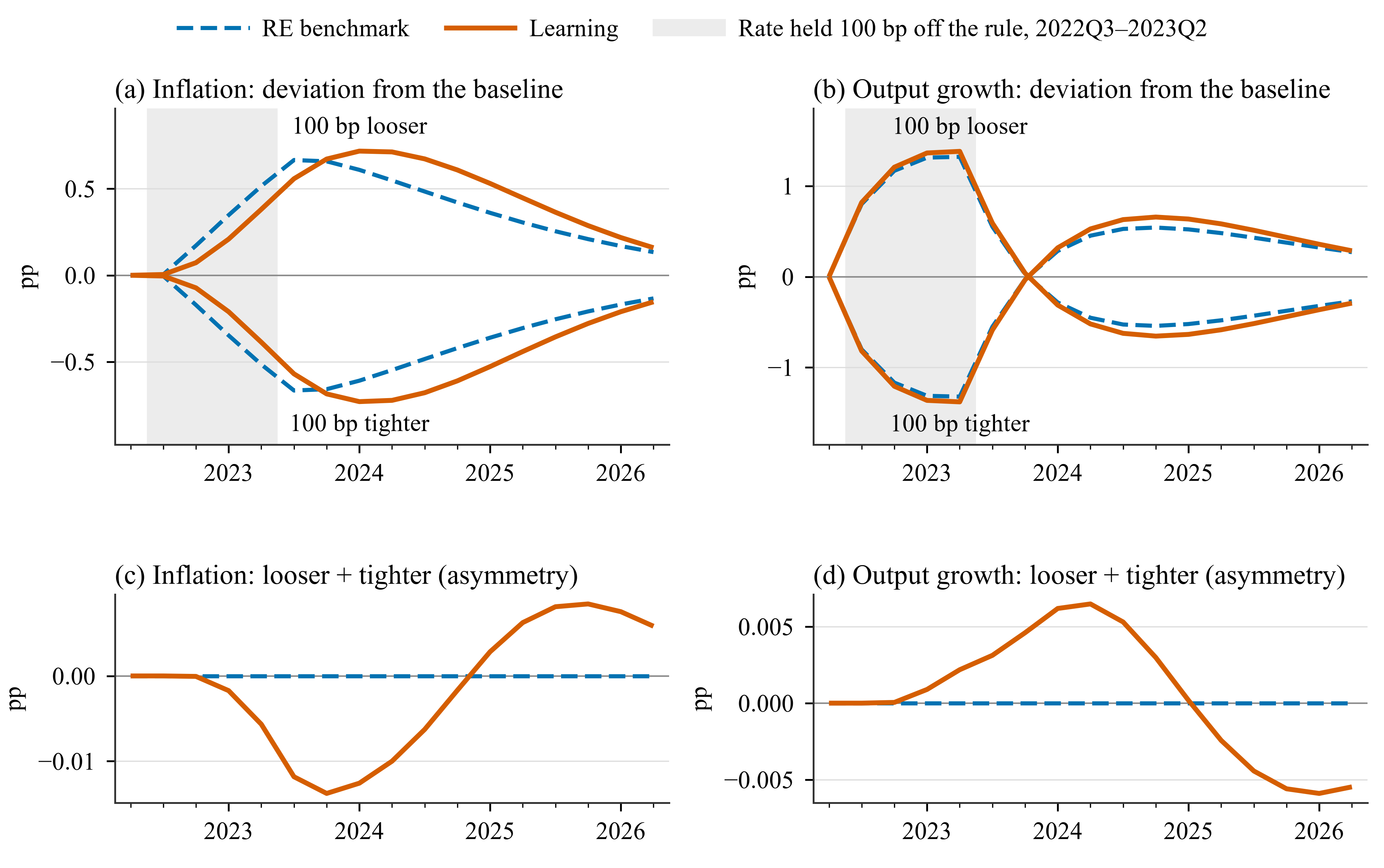
Deviations from Application 1 (pp of annualised rates) when the rate is held 100 bp a year below or above the Taylor rule in 2022Q3-2023Q2 (shaded). Top: inflation and output growth. Bottom: looser + tighter, which is zero when the responses are symmetric.

Variable	Statistic	RE, looser	Learning, looser	Learning, tighter	Looser + tighter
Inflation	largest effect	+0.666 (2023Q3)	+0.717 (2024Q1)	−0.730 (2024Q1)	−0.0138 (2023Q4)
	average effect	+0.366	+0.413	−0.415	−0.0015
Output growth	largest effect	+1.322 (2023Q2)	+1.382 (2023Q2)	−1.380 (2023Q2)	+0.0065 (2024Q2)
Policy rate	largest effect	−1.735 (2023Q2)	−1.817 (2023Q2)	+1.815 (2023Q2)	−0.0099 (2024Q2)
Learners' share in force	largest effect		+0.0244 (2024Q3)	−0.0295 (2024Q2)	−0.0053 (2024Q2)

• Learning delays the inflation response and makes it slightly larger: the peak effect of looser policy is +0.72 pp in 2024Q1 against +0.67 pp in 2023Q3 under RE.
• The asymmetry is small: at most 0.014 pp of inflation, about 2% of the effect. Under RE the two responses are exact mirror images (to 6e-14, check C3a).
• It comes from the learning states. Looser policy raises the learners' share in force by up to 0.024; tighter policy lowers it by up to 0.030.
• The policy-rate effect includes the rule's own response to the higher or lower inflation.

Variations

% 50 bp a year instead of 100 bp
cfg = a3_loose_learn(); cfg.id = 'a3_loose50_learn'; cfg.conditions.values = -0.125;
hetlearn.run(cfg);

% Put the observed policy rate itself on a path (level condition, % per quarter)
cfg = a1_learn(); cfg.id = 'a3_path_learn';
cfg.conditions = struct('variable', 'robs', 'shock', 'em', ...
    'dates', qq(2022, 3):qq(2023, 2), 'values', [0.5 0.8 1.1 1.2], ...
    'type', 'level', 'reference', 'self');
hetlearn.run(cfg);

More on conditions: Forecasts, shocks and conditions.