Application 5: density forecasts

Question. Application 1 assumes zero shocks. How wide is the range of outcomes when supply (mark-up) or demand shocks keep hitting the economy, and does learning change it?

Scenario files

scenarios/sw07/app5_density/:

function cfg = a5_markup_re()
cfg = a1_re();
cfg.id = 'a5_markup_re';
cfg.density.enabled = true;
cfg.density.shocks = {'epinf', 'ew'};      % price and wage mark-up shocks
cfg.density.sigma = 'calibrated';         % the model's std_<shock>
cfg.density.method = 'normal';
cfg.density.ndraws = 500;
cfg.density.seed = 0;
end

function cfg = a5_demand_re()
cfg = a5_markup_re();
cfg.id = 'a5_demand_re';
cfg.density.shocks = {'eb', 'eg', 'eqs'};  % risk premium, government spending, investment
end

function cfg = a5_markup_learn()
cfg = a1_learn();
d = a5_markup_re();
cfg.id = 'a5_markup_learn';
cfg.density = d.density;                   % the same draws as the RE run
cfg.compare_with = {'a5_markup_re'};
end

a5_demand_learn copies the density block of a5_demand_re the same way.

Each draw adds random shocks on top of the scenario (here, zero shocks) in every forecast quarter. An RE density without conditions takes a fast path: one linear simulation per draw (about 30 seconds for 500 draws). A learning density re-runs the quarter-by-quarter forecast for each draw, so beliefs and shares respond to the drawn shocks (about 0.5-0.7 seconds per draw).

run_applications('app5')        % about 14 minutes

Outputs, besides the usual files: results/<id>/density.mat, density_quantiles.csv (variable, date, quantile, value in model and report units) and density_events.csv (one row per draw: status and facility events).

Results

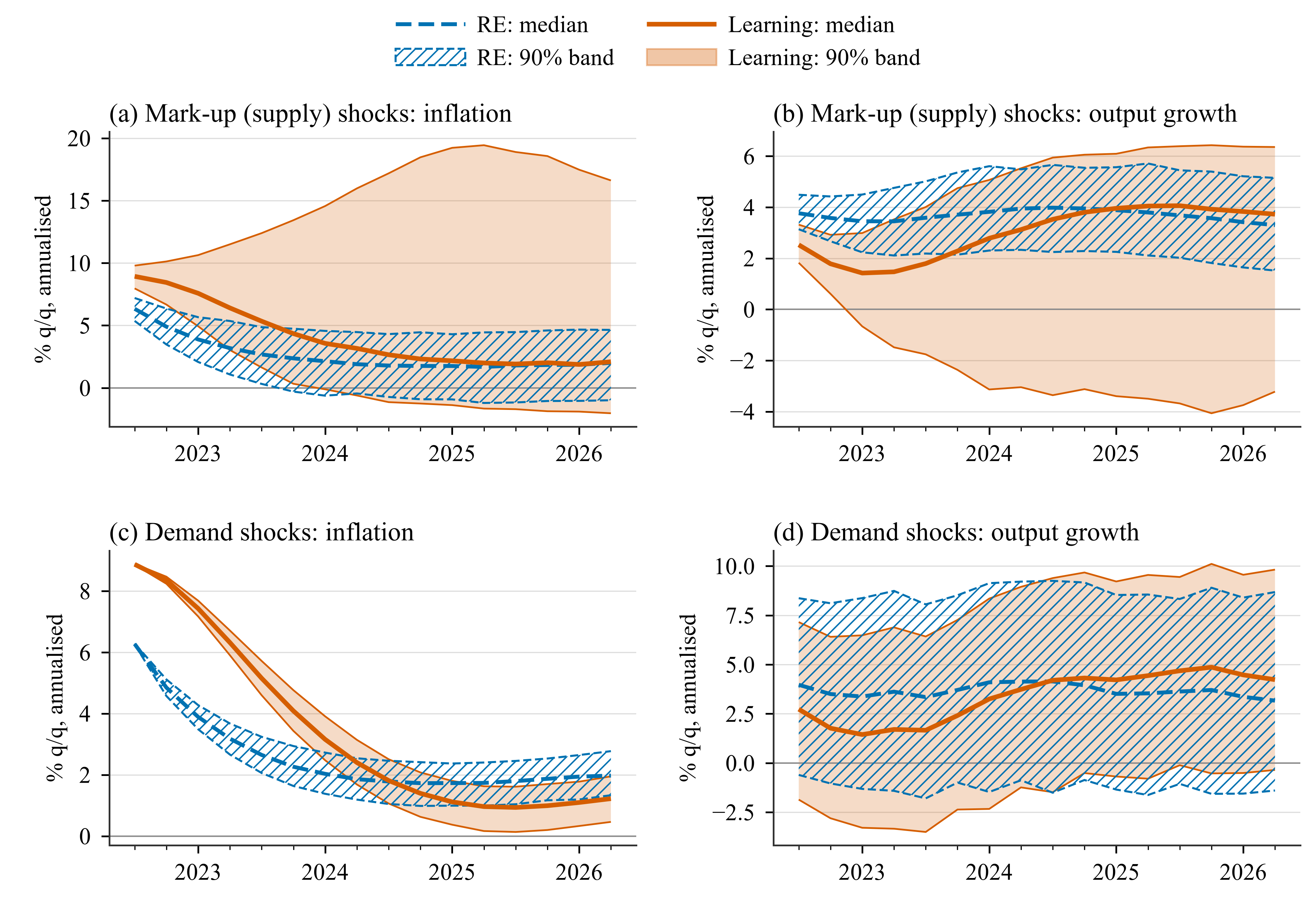
90% bands (5th-95th percentiles) and medians of 500 forecasts from the 2022Q2 peak. Top: mark-up shocks; bottom: demand shocks. RE band hatched, learning band filled.

Shocks	Variable	Average 90% band width, RE (pp)	Learning (pp)
Mark-up (epinf, ew)	inflation	4.76	14.59
	output growth	3.02	7.51
	policy rate	2.85	10.71
Demand (eb, eg, eqs)	inflation	1.18	1.16
	output growth	9.92	10.03

• Mark-up shocks: learning triples the inflation band. The learning distribution is skewed upwards: inflation shocks feed the learners' explosive AR(1) beliefs (\(\beta = 1.061\) at the origin) and their share. In 2026Q2 the learning band runs from −2.0% to 16.6% (RE: −1.0% to 4.6%).
• Demand shocks: the bands are about the same under learning and RE, because these shocks move inflation little.
• The facility matters in the tail. It acts in 23 of the 500 learning mark-up draws (46 quarters with beliefs reverted, 13 with shares kept) and in none of the demand draws. All draws are used.

Variations

% Shock standard deviations from the RE-smoothed shocks of 1966-2019
cfg = a5_markup_learn(); cfg.id = 'a5_markup_learn_sm';
cfg.density.sigma = 'smoothed';
cfg.density.sigma_range = [qq(1966, 1), qq(2019, 4)];
hetlearn.run(cfg);

% Bootstrap whole quarters of smoothed shocks, 200 draws, keep every draw
cfg = a5_markup_learn(); cfg.id = 'a5_markup_learn_bs';
cfg.density.method = 'bootstrap';
cfg.density.demean = true;
cfg.density.ndraws = 200;
cfg.density.keep_draws = true;
hetlearn.run(cfg);

All density options: Density forecasts.