Perceived laws of motion (PLMs)

A PLM is the learners' forecasting model: a linear regression of a variable on lags of itself or of other variables, whose coefficients they re-estimate each quarter.

Option	Values (default first)	Meaning
beliefs.plm.default	'ar1', 'ar2', 'ar1_noconst', 'var1'	PLM of every learning variable without its own entry; 'var1' = one VAR(1) over the learning set
beliefs.plm.by_var.<x>	a shorthand ('ar1', 'ar2', 'ar1_noconst') or struct('regressors', {...}, 'constant', true)	PLM of one variable. An entry for a variable that does not learn sets its auxiliary PLM
beliefs.plm.derived.<name>	text	A regressor defined as a linear expression in model variables, e.g. 'y - yf'; it becomes a model variable
beliefs.plm.var	struct('variables', {{}}, 'lags', 1, 'constant', true)	A VAR PLM over a cellstr of variables or 'learning' (the learning set)

How a PLM forecasts

A PLM equation for variable \(v\) is

\[ v_t = \alpha_v + \sum_j \beta_{v,j}\, u_{j,t-l_j} + \varepsilon_t, \qquad l_j \ge 1 . \]

With beliefs.info = 'lagged' the learners see data up to t-1, so for the one-step-ahead forecast of \(x_{t+1}\) they iterate the PLMs forward from t-1, replacing every unobserved regressor by its own PLM forecast. For the AR(1): \(\alpha + \beta(\alpha + \beta x_{t-1})\). With 'current' they iterate from t: \(\alpha + \beta x_t\).

Belief parameters are named after the PLM: alpha_<x> and beta_<x> for an AR(1) with a constant; alpha_<x> and beta_<x>__<u>_l<lag> for anything else (for example beta_pinf__ygap_l1). They appear under these names in res.learning.<x> and learning.csv.

Examples

% AR(2) learners (model variant v2_ar2)
cfg = a1_learn(); cfg.id = 'v2_ar2';
cfg.beliefs.plm.default = 'ar2';

% AR(1) without constant: only the persistence is learned (v2_ar1nc)
cfg = a1_learn(); cfg.id = 'v2_ar1nc';
cfg.beliefs.plm.default = 'ar1_noconst';

% Inflation on lagged inflation, output gap and policy rate (v2_reg)
cfg = a1_learn(); cfg.id = 'v2_reg';
cfg.beliefs.plm.derived.ygap = 'y - yf';
cfg.beliefs.plm.by_var.pinf = struct('regressors', {{'pinf{-1}', 'ygap{-1}', 'r{-1}'}}, 'constant', true);

% VAR(1) in inflation, output gap and policy rate (v2_var3)
cfg = a1_learn(); cfg.id = 'v2_var3';
cfg.beliefs.plm.derived.ygap = 'y - yf';
cfg.beliefs.plm.var = struct('variables', {{'pinf', 'ygap', 'r'}}, 'lags', 1, 'constant', true);

% VAR(1) in the 12 forward-looking variables of SW07 (v2_var12)
cfg = a1_learn(); cfg.id = 'v2_var12';
cfg.beliefs.plm.var = struct('variables', ...
    {{'invef', 'rkf', 'pkf', 'cf', 'labf', 'inve', 'pinf', 'rk', 'pk', 'c', 'lab', 'w'}}, ...
    'lags', 1, 'constant', true);

% One PLM per variable with a shorthand
cfg = a1_learn(); cfg.id = 'a1_byvar_ar2';
cfg.beliefs.plm.by_var.pinf = 'ar2';

% Mean-only PLM: the forecast is the learned mean (adaptive expectations)
cfg = a1_learn(); cfg.id = 'a1_mean_only';
cfg.beliefs.plm.by_var.pinf = struct('regressors', {{}}, 'constant', true);

Run any of them with hetlearn.run(cfg).

Rules

• Regressors are lags. Write them as name{-k} with k >= 1.
• Auxiliary PLMs. A regressor that is not itself a learning variable gets an auxiliary PLM (an AR(1) with constant by default), learned by the same RLS, so the learners can iterate the system forward. In v2_reg, ygap and r get auxiliary AR(1)s. Set an auxiliary PLM with a by_var entry for that variable.
• VARs. VAR members that do not learn become auxiliary VAR equations; only the learning variables' expectations use the VAR forecast. VAR members take no by_var entry.
• 'var1' builds a VAR(1) over the whole learning set. It cannot be combined with beliefs.plm.var.variables (an error).
• Derived regressors must be linear expressions in model variables; each becomes a model variable with that definition.
• Blocks. PLM equations linked through their regressors form a block (a VAR is one block; separate AR(1)s are separate blocks). The projection facility 'plm_alm' judges each block by its largest root.
• Generated files. The default AR(1) PLM uses generated/<name>_ext_ar1.model; any other PLM spec gets its own file, tagged with a hash of the spec (<name>_ext_p<8 hex>.model), and its own RE filter cache.

In the project

Model variant 2 runs Application 1 with each PLM. Averages over 2022Q3-2026Q2:

PLM for inflation	Scenario	Inflation (%)	Rate (%)	Output growth (%)	Share 2022Q2	Peak share	Largest root 2022Q2	Mean root 1966-2022
RE benchmark	a1_re	2.59	4.53	3.69
AR(1), baseline	a1_learn	3.45	5.42	3.39	0.591	0.685	1.061	0.747
AR(1), no constant	v2_ar1nc	3.25	5.18	3.46	0.611	0.651	1.031	0.883
AR(2)	v2_ar2	3.69	5.63	3.29	0.599	0.760	1.086	0.806
Regression on \(\pi, x, r\)	v2_reg	2.56	4.51	3.78	0.601	0.664	1.039	0.985
VAR(1) in \(\pi, x, r\)	v2_var3	2.57	4.53	3.77	0.598	0.659	1.030	0.953
VAR(1) in 12 variables	v2_var12	3.19	5.09	3.46	0.611	0.618	1.004	0.998

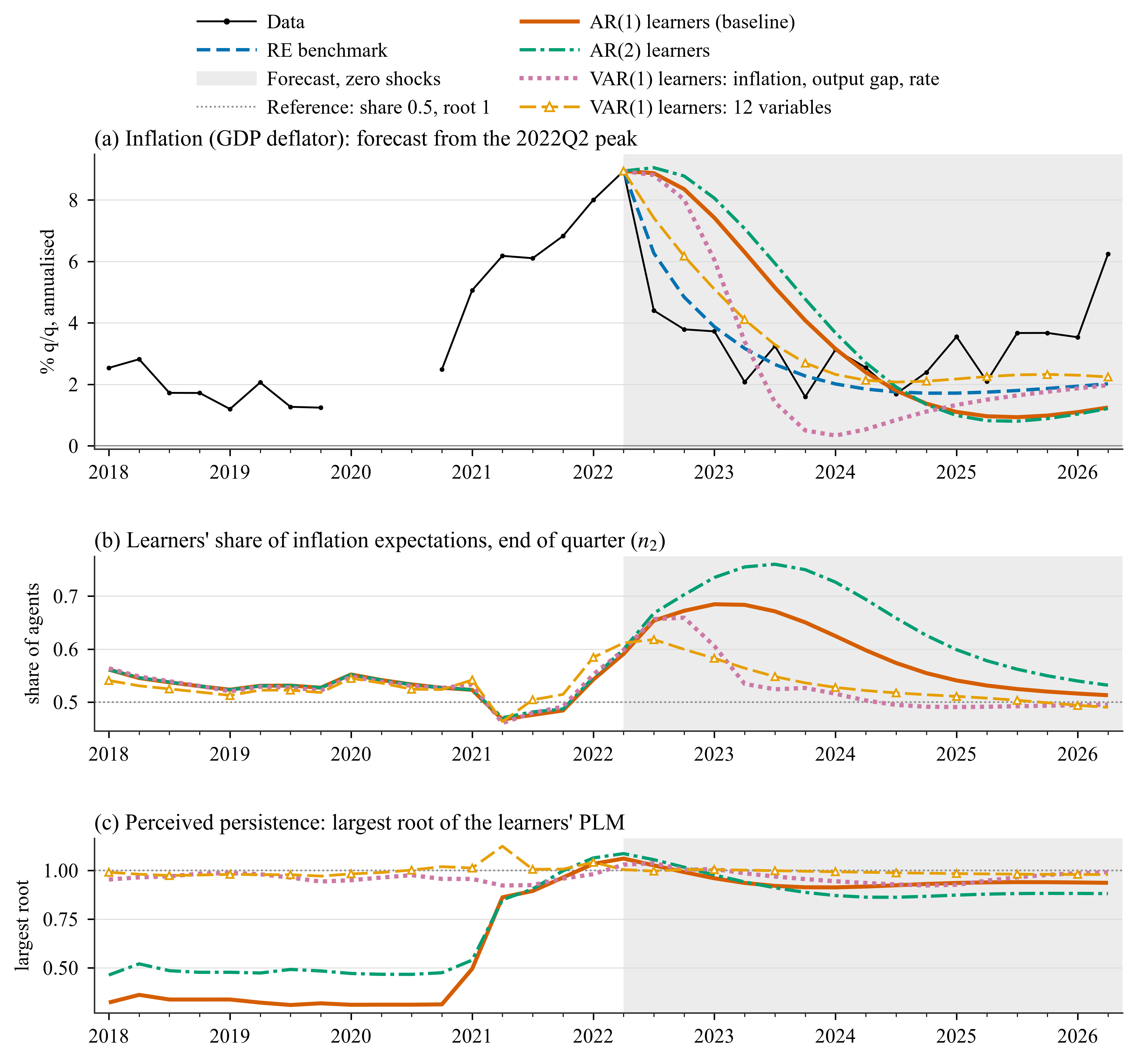
Inflation, the learners' share and the largest root of the PLM, four PLMs.

Every PLM has a largest root at or above 1 at the 2022Q2 origin, so none has a finite perceived mean there. PLMs that include the output gap and the policy rate (v2_reg, v2_var3) bring inflation down about as fast as RE; AR PLMs, which see only past inflation, keep it higher for longer. The VAR learners perceive inflation as close to a unit root over the whole history (mean root 0.95-1.00). No projection-facility event occurs in any of these runs.